OLAP Graph

I want to present a quick study I’ve done with my colleague João Raimundo about an experiment around OLAP1 operations using a Graph.
We call it: The “Graph” Kimball Presentation2.
- Why Graphs?
- We found a NoSQL Graph-based OLAP Analysis paper3 that really caught our eye and we wanted to see how this version of OLAP analysis compares to the usual tabular OLAP approach.
We then purpose how to correctly use a Graph for Cube Architecture and OLAP Operations.
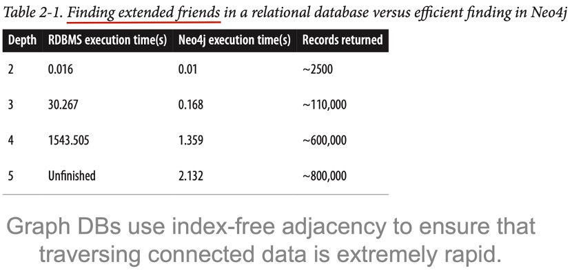
I leave this table as an initial reference of how powerful graph-based databases can be, in particular Neo4J which is the same one that is used on this study. Do note that the example presented is a motivation for graph-based databases so the example is a finger-picked one.
Graph Architecture
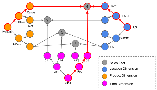
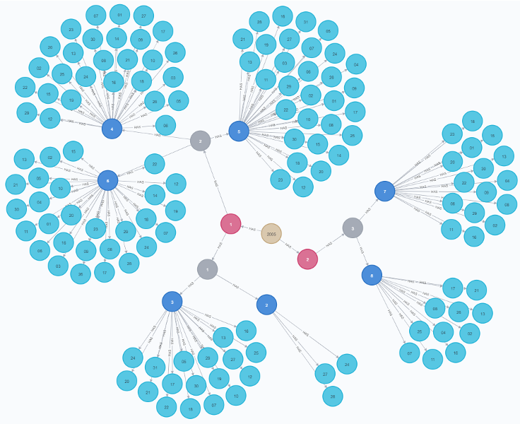
We follow the NoSQL Graph-based OLAP Analysis paper’s architecture which is presented in the image below.
In here we can easily identify Dimension Nodes that are created in a snowflake architecture (should we compare it to the tabular version), and Fact Nodes where we can spot them out by seeing where all the connections intersect.
It is important to say as well that we can define levels of our Dimensions with new nodes instead of the tabular version where we would need to add a new column.
We can identify three Dimensions: Location, Product, and Time as well as the Fact nodes with grey color.
Practical Example
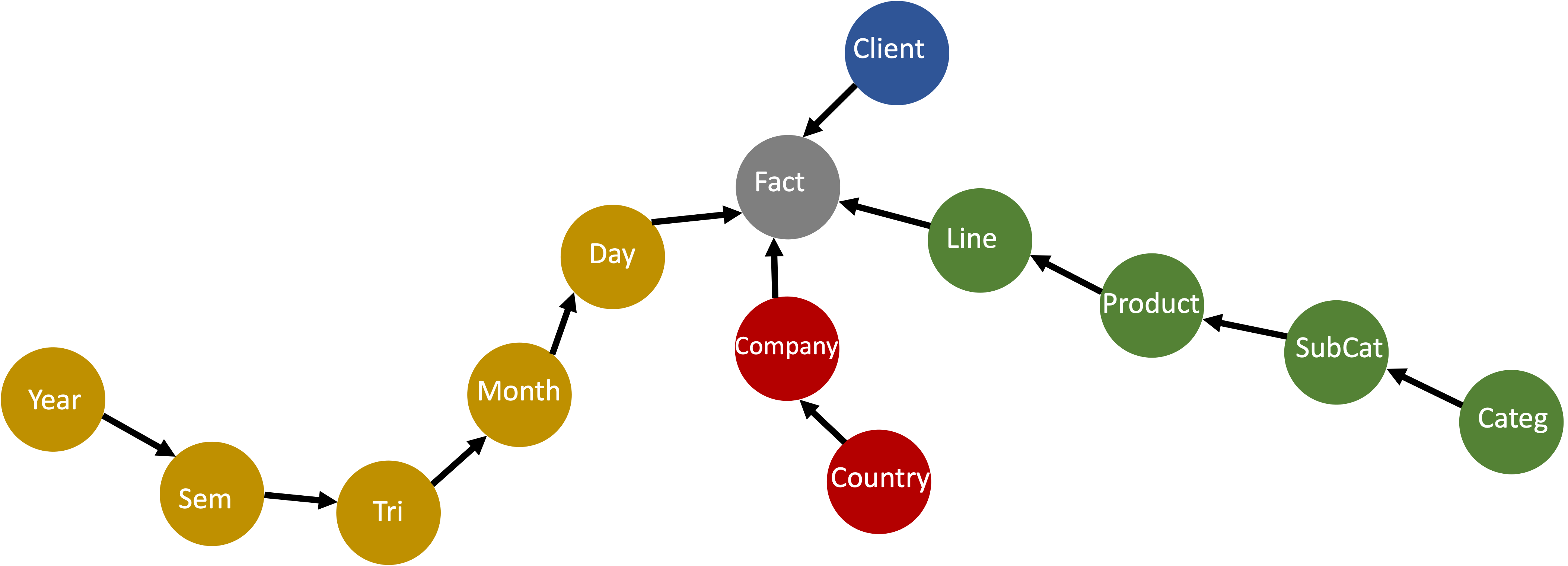
To easily show you how powerful this Graph-based OLAP can be, we created a Hypervending Data Warehouse to use on the demonstrations that will follow.
We can notice that each Dimension is a node, and the same can be said for the Facts.
To make it even more interesting, we can define the levels of each dimension very easily and they can be identified almost without effort by following the archs between the nodes. These archs have to be unidirectional.
Facts and Measures
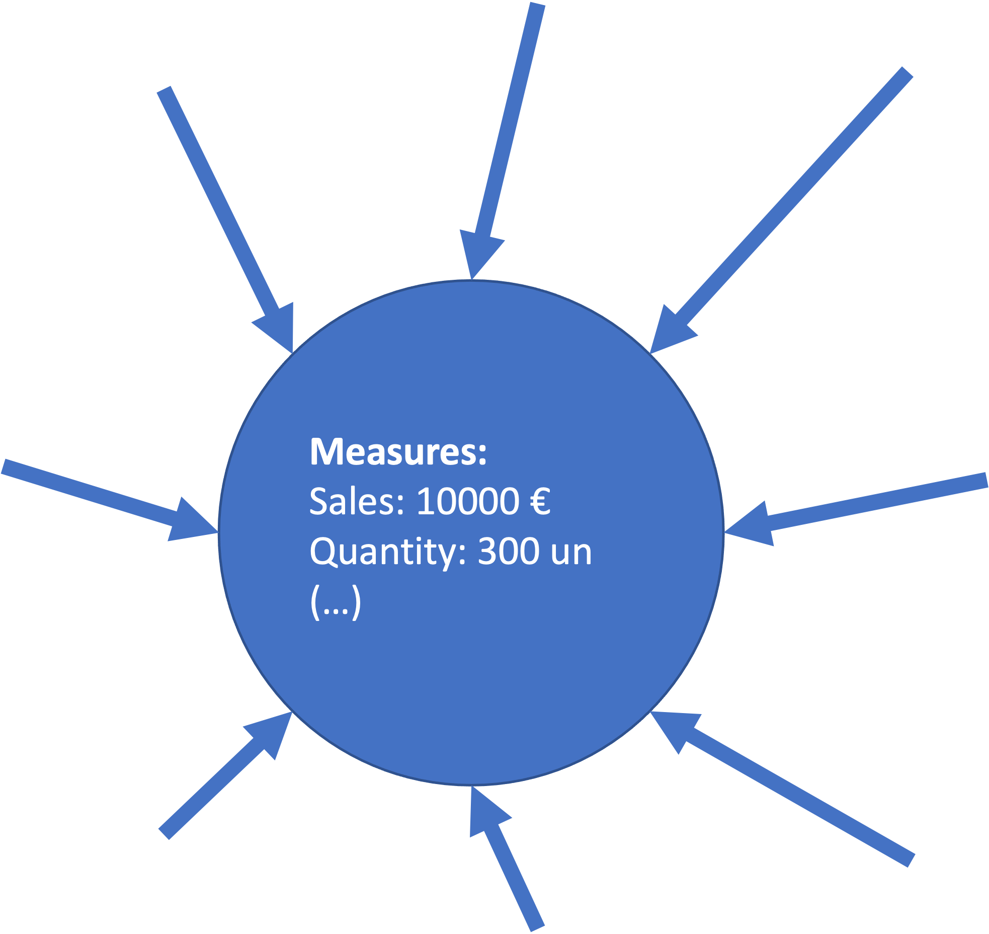
A Fact Node is identified by the archs directed at it. There is a direct relation between the number of Dimensions and the centrality of the Node.
The Measures are indicated in the attributes of the Fact Nodes.
We can have different types of Fact Node in our OLAP Graph, utilizing the same dimensions. These can be seen as a different data-marts.
Degree and Dimensions
One thing that we can immediately understand from using a graph approach for the OLAP Analysis is that we can identify, without effort, the nodes with the most importance.
The nodes with more connections are the most “popular node”. As we can see from this example, we can identify which months (in grey) are the most popular months for sales
Slow-changing Dimensions
In our more tabular SQL-driven approach, slow changing dimensions require a special type of treatment, and it can easily be the reason for an over-growth of our dimension tables.
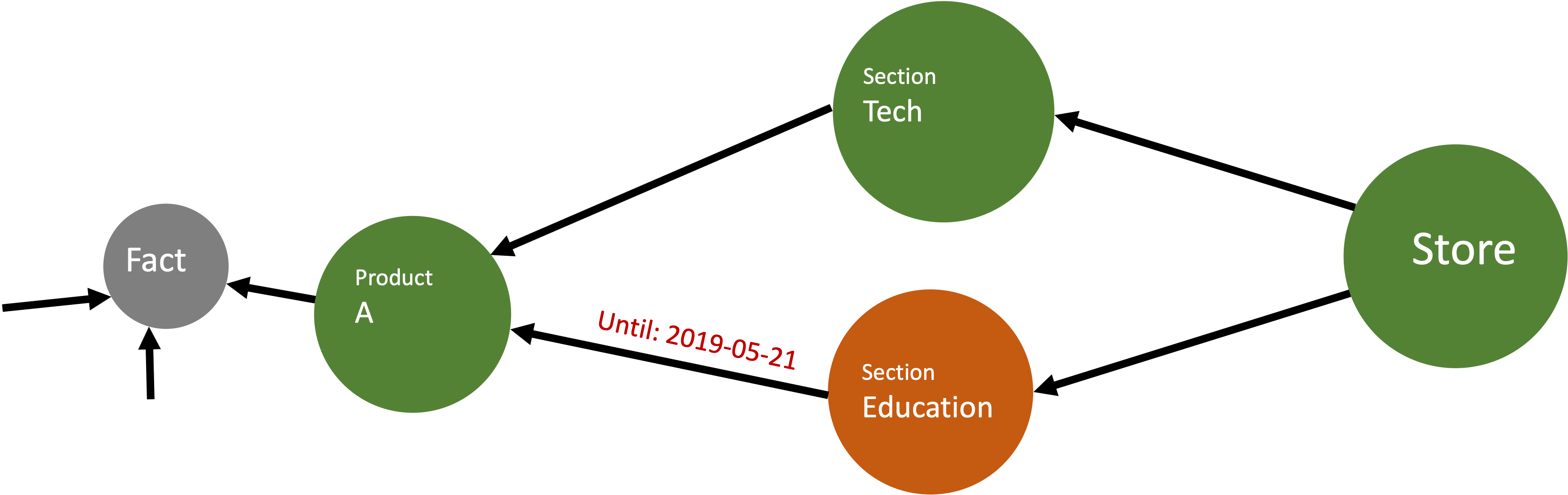
With the graph approach, the only thing we need to do is save the property of the versioning in the arch that connects two dimensions.
The arch saves the last time that connection was true in a timestamp, allowing us to query it easily using cypher4, as follows:
1
2
3
MATCH (store:Store {name: "Super"})-[]->(sec:Section)-[arch:HAS]->(prod:Product {name: "A"})
WHERE arch.date >= 2019-05-21
RETURN store, sec, prod
Operations
OLAP allows us to execute some important operations such as Slice, Dice, Drill-Down, Roll-Up.
I will be showing how the same operations can be done using an OLAP Graph instead with the help of illustrative images and some Cypher code
Slice
Get Sales made in “Lisboa”.
1
2
MATCH (f:Fact)<-[]-(c:Customer {name: "Lisboa"})
RETURN f, c
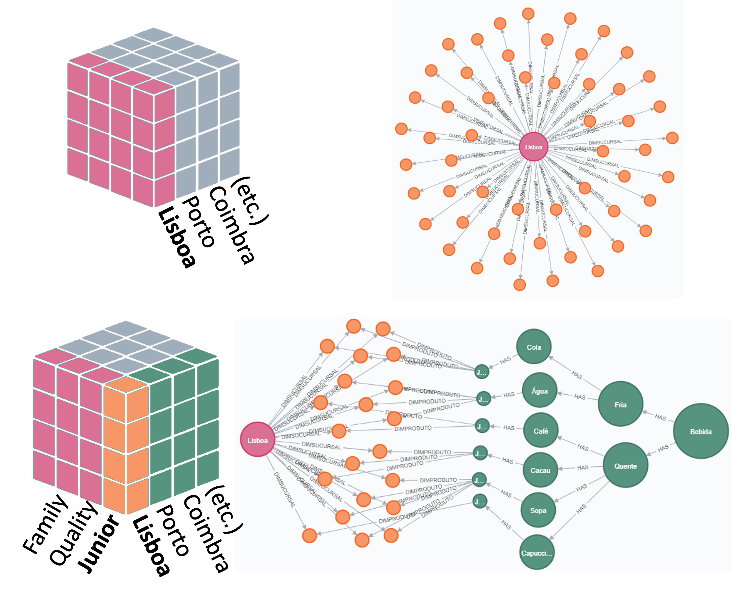
Get Sales made in “Lisboa” and Product line = “Junior”.
1
2
3
MATCH (f:Fact)<-[]-(c:Customer {name: "Lisboa"})
MATCH (f)<-[]-(l:Line {name: "Junior"})<-[]-(p)<-[]-(sub)<-[]-(cat)
RETURN f, c, l, p, sub, cat
Dice
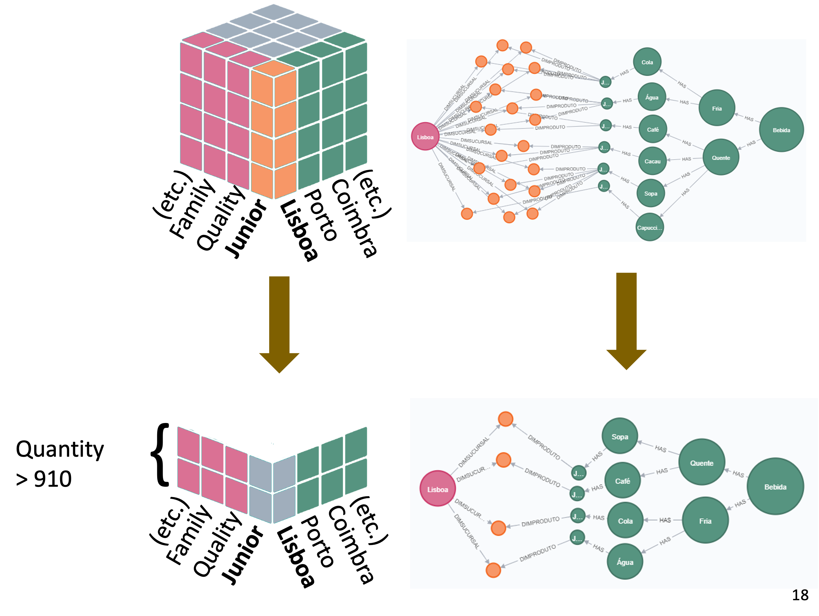
Get Sales made in “Lisboa” and Product line = “Junior” WHERE quantity is larger than 910.
1
2
3
4
MATCH (f:Fact)<-[]-(c:Customer {name: "Lisboa"})
MATCH (f)<-[]-(l:Line {name: "Junior"})<-[]-(p)<-[]-(sub)<-[]-(cat)
WHERE f.quantity >= 910
RETURN f, c, l, p, sub, cat
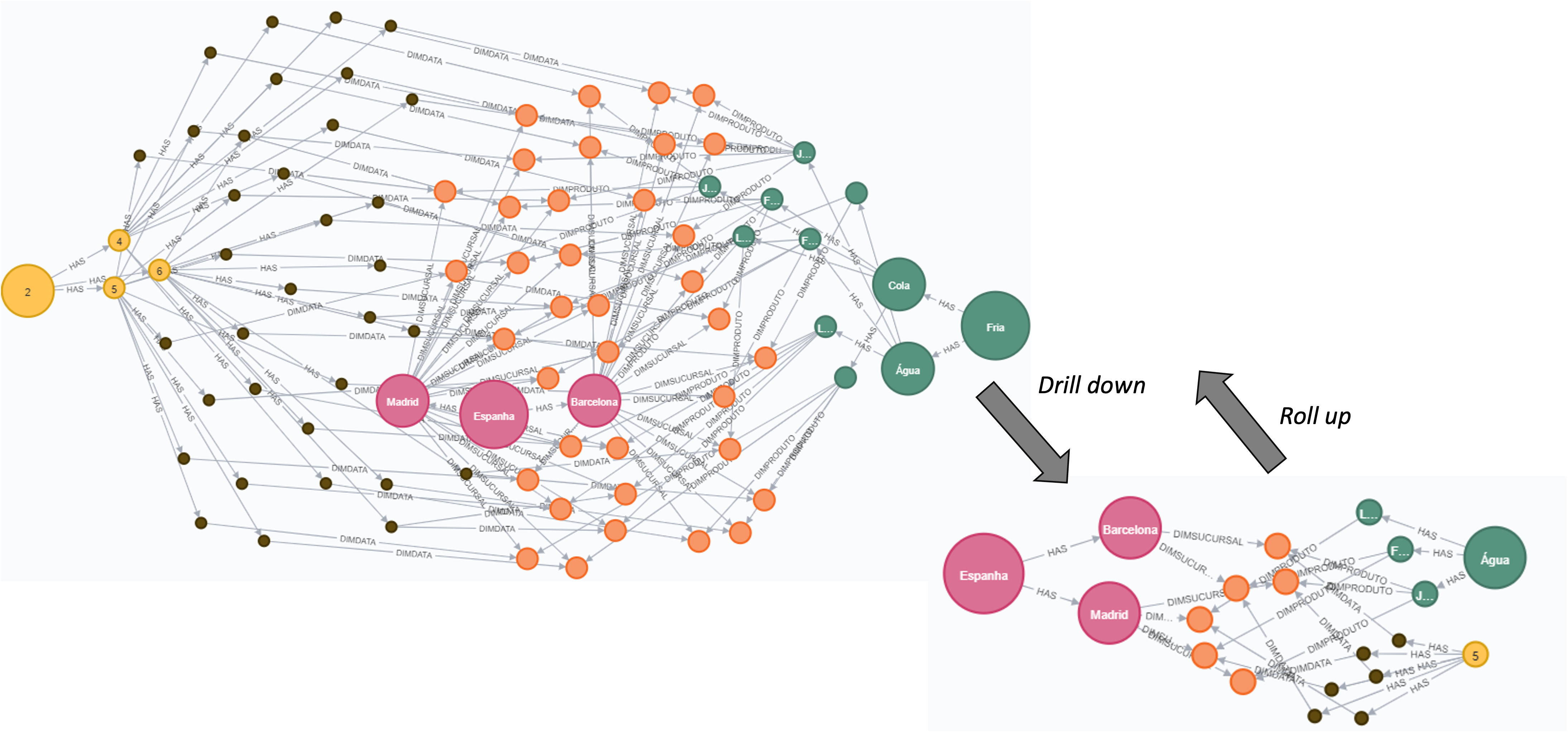
Roll-up and Drill-Down
Get Sales made in “Spain” with sub-category = “Cold” in the 2nd trimester.
1
2
3
4
MATCH (f:Fact)<-[]-(s)<-[]-(co:Country {name: "Spain"})
MATCH (f)<-[]-(l)<-[]-(prod)<-[]-(sub:SubCategory {name: "Cold"})
MATCH (f)<-[]-(d)<-[]-(m)<-[]-(tri:Trimester {_: 2})
RETURN f, s, co, l, prod, d, m, sub, tri
Get Sales made in “Spain” with product = “Coffee” in the 5th month
1
2
3
4
MATCH (f:Fact)<-[]-(s)<-[]-(co:Country {name: "Spain"})
MATCH (f)<-[]-(l)<-[]-(prod:Product {name: "Coffee"})
MATCH (f)<-[]-(d)<-[]-(m:Month {_: 5})
RETURN f, s, co, l, prod, d, m
Exploration and Conclusion
Given all that has been said, this is our final demonstration of what a Graph approach can give you. Sorry for bad resolution that Giphy allows me to have.
With a Graph OLAP “cube” and Neo4J we can do our exploratory analysis in a way that is unimaginable for the SQL approach.
Is it something that can be used to actually study the data? We say YES! but I’ll leave that answer up to you and your projects where you can hopefully get some inspiration from here :)